Ram Rallabandi

This dataset (source) includes 44,066 results of international football matches starting from the very first official match in 1872 up to 2022. The matches range from FIFA World Cup to FIFI Wild Cup to regular friendly matches. The matches are strictly men’s full internationals and the data does not include Olympic Games or matches where at least one of the teams was the nation’s B-team, U-23 or a league select team.

Task 1: Import and prepare the dataset

• Import the pandas package with the usual alias.

In [1]:

# Import the pandas package with the usual alias
import pandas as pd

• Read "results.csv". Assign to results.
• Convert the date column to a datetime.
• Get the year component of the date column; store in a new column named year.

In [2]:

# Read results.csv. Assign to results.
results = pd.read_csv("results.csv")
results.head()
results.dtypes
# Convert the date column to a datetime
results['date'] = pd.to_datetime(results['date'])
results.dtypes
# Get the year component of date column; store in a new column named year 
results['year'] = results['date'].dt.year
results.head()

# See the result
results

Out[2]:

	date	home_team	away_team	home_score	away_score	tournament	city	country	neutral	year
0	1872-11-30	Scotland	England	0	0	Friendly	Glasgow	Scotland	False	1872
1	1873-03-08	England	Scotland	4	2	Friendly	London	England	False	1873
2	1874-03-07	Scotland	England	2	1	Friendly	Glasgow	Scotland	False	1874
3	1875-03-06	England	Scotland	2	2	Friendly	London	England	False	1875
4	1876-03-04	Scotland	England	3	0	Friendly	Glasgow	Scotland	False	1876
…	…	…	…	…	…	…	…	…	…	…
44061	2022-10-22	Saudi Arabia	North Macedonia	1	0	Friendly	Abu Dhabi	United Arab Emirates	True	2022
44062	2022-10-23	Qatar	Guatemala	2	0	Friendly	Málaga	Spain	True	2022
44063	2022-10-26	Saudi Arabia	Albania	1	1	Friendly	Abu Dhabi	United Arab Emirates	True	2022
44064	2022-10-27	Qatar	Honduras	1	0	Friendly	Marbella	Spain	True	2022
44065	2022-10-30	Saudi Arabia	Honduras	0	0	Friendly	Abu Dhabi	United Arab Emirates	True	2022

44066 rows × 10 columns

Task 2: Get the FIFA World Cup data

• Using results, count the number of rows of each tournament value.
• Convert the results to a DataFrame for nicer printing.

In [3]:

# Count the number of rows for each tournament; convert to DataFrame
results.value_counts('tournament')
#convert to Dataframe
results.value_counts('tournament').to_frame("num_maatches")

Out[3]:

	num_maatches
tournament
Friendly	17427
FIFA World Cup qualification	7774
UEFA Euro qualification	2593
African Cup of Nations qualification	1932
FIFA World Cup	900
…	…
AFF Championship qualification	2
TIFOCO Tournament	1
FIFA 75th Anniversary Cup	1
Copa Confraternidad	1
Real Madrid 75th Anniversary Cup	1

139 rows × 1 columns

• Query for the rows where tournament is equal to “FIFA World Cup”

In [4]:

# Query for the rows where tournament is equal to "FIFA World Cup"
world_cup_res= results.query("tournament=='FIFA World Cup'")

# See the results
world_cup_res

Out[4]:

	date	home_team	away_team	home_score	away_score	tournament	city	country	neutral	year
1311	1930-07-13	Belgium	United States	0	3	FIFA World Cup	Montevideo	Uruguay	True	1930
1312	1930-07-13	France	Mexico	4	1	FIFA World Cup	Montevideo	Uruguay	True	1930
1313	1930-07-14	Brazil	Yugoslavia	1	2	FIFA World Cup	Montevideo	Uruguay	True	1930
1314	1930-07-14	Peru	Romania	1	3	FIFA World Cup	Montevideo	Uruguay	True	1930
1315	1930-07-15	Argentina	France	1	0	FIFA World Cup	Montevideo	Uruguay	True	1930
…	…	…	…	…	…	…	…	…	…	…
40293	2018-07-07	Russia	Croatia	2	2	FIFA World Cup	Sochi	Russia	False	2018
40294	2018-07-10	France	Belgium	1	0	FIFA World Cup	Saint Petersburg	Russia	True	2018
40295	2018-07-11	Croatia	England	2	1	FIFA World Cup	Moscow	Russia	True	2018
40296	2018-07-14	Belgium	England	2	0	FIFA World Cup	Saint Petersburg	Russia	True	2018
40297	2018-07-15	France	Croatia	4	2	FIFA World Cup	Moscow	Russia	True	2018

900 rows × 10 columns

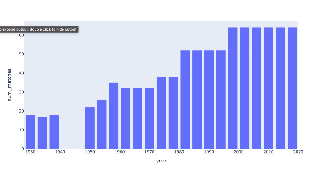
Task 3: Your turn: How many matches in every world cup?

• Using world_cup_res, count the number of rows of each year value.
• Convert the results to a DataFrame for nicer printing.

In [5]:

# Count the number of rows for each year; convert to DataFrame

matches_per_year= world_cup_res.value_counts("year").to_frame("num_matches")

# See the results
matches_per_year

#additional
# size vs count - both are same NaNs are accounted in size

world_cup_res.groupby(by='year').size().to_frame("num_matches")

Out[5]:

year	num_matches
1930	18
1934	17
1938	18
1950	22
1954	26
1958	35
1962	32
1966	32
1970	32
1974	38
1978	38
1982	52
1986	52
1990	52
1994	52
1998	64
2002	64
2006	64
2010	64
2014	64
2018	64

• Import the plotly.express package using the alias px.

In [6]:

# Import the plotly express package using the alias px
import plotly.express as px

• Using matches_per_year, draw a bar plot of num_matches.

The year is in the index and will automatically be used for the x-axis.

In [7]:

# Using matches_per_year, draw a bar plot of num_matches
px.bar(matches_per_year, y="num_matches")

Task 4: Which games had the highest goal difference?

• Add a goal_difference column as the absolute value of the home score minus the away score.
• Query for rows where the goal difference equals the maximum goal difference.

In [8]:

# Add a goal_difference column as the absolute value of the home score minus the away score
# Query for rows where the goal difference equals the maximum goal difference
world_cup_res\
.assign(goal_difference = lambda match: (match['home_score'] - match['away_score']).abs())\
.query('goal_difference==goal_difference.max()')

Out[8]:

	date	home_team	away_team	home_score	away_score	tournament	city	country	neutral	year	goal_difference
3667	1954-06-17	Hungary	South Korea	9	0	FIFA World Cup	Zürich	Switzerland	True	1954	9
9208	1974-06-18	Yugoslavia	DR Congo	9	0	FIFA World Cup	Gelsenkirchen	Germany	True	1974	9
12555	1982-06-15	Hungary	El Salvador	10	1	FIFA World Cup	Elche	Spain	True	1982	9

Task 5: Your turn: Which game had the highest total number of goals?

• Add a total_goals column as the home score plus the away score.
• Query for rows where the total goals equals the maximum total goals.

In [9]:

# Add a total_goals column as the  home score plus the away score
# Query for rows where the total goals equals the maximum total goals

world_cup_res\
	.assign(total_goals = lambda match : match["home_score"] +match["away_score"])\
.query('total_goals == total_goals.max()')

Out[9]:

	date	home_team	away_team	home_score	away_score	tournament	city	country	neutral	year	total_goals
3680	1954-06-26	Switzerland	Austria	5	7	FIFA World Cup	Lausanne	Switzerland	False	1954	12

Task 6: Which country scored the most goals?

Step 1: Calculate the home goals by country

• Using world_cup_res, get the home_team and home_score columns.
• Rename as team and score.

In [10]:

# Get the home_team and home_score columns
# Rename as team and score
home_goals = world_cup_res.filter(['home_team','home_score'])\
	.rename(columns={'home_team':'home', 'home_score':'score'})


# See the result
home_goals

Out[10]:

	home	score
1311	Belgium	0
1312	France	4
1313	Brazil	1
1314	Peru	1
1315	Argentina	1
…	…	…
40293	Russia	2
40294	France	1
40295	Croatia	2
40296	Belgium	2
40297	France	4

900 rows × 2 columns

Your turn: Step 2: Calculate the away goals by country

• Using world_cup_res, get the away_team and away_score columns.
• Rename as team and score.

In [11]:

# Get the away_team and away_score columns
# Rename as team and score

away_goals = world_cup_res.filter(['away_team','away_score'])\
	.rename(columns={'away_team':'team', 'away_score':'score'})
# See the result
away_goals

Out[11]:

	team	score
1311	United States	3
1312	Mexico	1
1313	Yugoslavia	2
1314	Romania	3
1315	France	0
…	…	…
40293	Croatia	2
40294	Belgium	0
40295	England	1
40296	England	0
40297	Croatia	2

900 rows × 2 columns

Step 3: Combine the home and away totals

• Concatenate home_goals and away_goals.
• Group by team, as_index set to False.
• Calculate the total score.
• Rename the score column to total_goals.
• Sort the total goals so the country with the highest total shows on top.

In [12]:

# Concatenate home_goals and away_goals
# Group by team, as_index equal to False
# Get the total score
# Rename score to total_goals
# Sort by total_goals

total_goals_by_country=pd.concat([home_goals, away_goals])\
	.groupby(by='team', as_index=False)\
	.sum('score')\
	.rename(columns={"score":'total_goals'})\
	.sort_values("total_goals", ascending=False)


# See the result
total_goals_by_country

Out[12]:

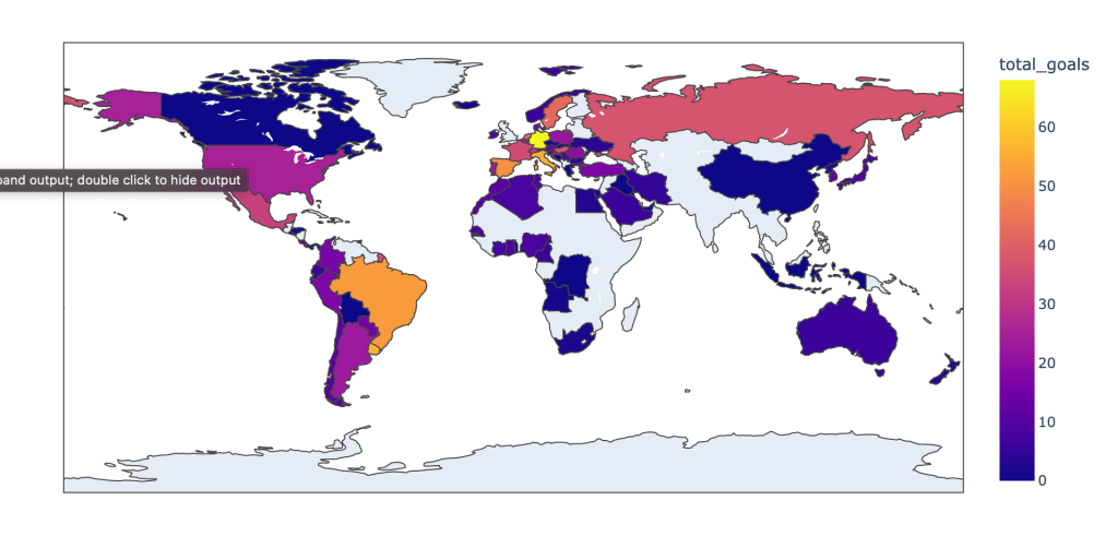
	team	total_goals
27	Germany	68
76	Uruguay	56
37	Italy	56
8	Brazil	52
66	Spain	50
…	…	…
19	DR Congo	0
34	Indonesia	0
11	Canada	0
13	China PR	0
70	Trinidad and Tobago	0

79 rows × 2 columns

Step 4: draw a map colored by number of goals

• Draw a plotly choropleth map, colored by total_goals, showing the team on hover.

In [13]:

# Draw a plotly choropleth map
px.choropleth(total_goals_by_country, 
              locations="team",
              locationmode="country names",
              color="total_goals",
               hover_name="team")

Extra: Does playing close to home matter?

Import the data

• Import the winners.csv file and add the winner for 2018 based on info you find online

In [14]:

# Import the data
# source = wikipedia 🙂
winner_2018 = pd.DataFrame({"year": [2018], "hosting_country": ["Russia"], "winning_country": ["France"]})
# source = https://www.kaggle.com/datasets/abecklas/fifa-world-cup
winners = pd.read_csv("winners.csv")[["Year", "Country", "Winner"]] \
			.replace('Germany FR', 'Germany', regex=False) \
			.rename(columns = {'Year': "year", 'Country': 'hosting_country', "Winner": "winning_country"}) \
			.append(winner_2018)

winners

/var/folders/q_/3r83m4b95gz1zx4qbfv56fmw0000gn/T/ipykernel_72195/4165530431.py:5: FutureWarning:

The frame.append method is deprecated and will be removed from pandas in a future version. Use pandas.concat instead.

Out[14]:

	year	hosting_country	winning_country
0	1930	Uruguay	Uruguay
1	1934	Italy	Italy
2	1938	France	Italy
3	1950	Brazil	Uruguay
4	1954	Switzerland	Germany
5	1958	Sweden	Brazil
6	1962	Chile	Brazil
7	1966	England	England
8	1970	Mexico	Brazil
9	1974	Germany	Germany
10	1978	Argentina	Argentina
11	1982	Spain	Italy
12	1986	Mexico	Argentina
13	1990	Italy	Germany
14	1994	USA	Brazil
15	1998	France	France
16	2002	Korea/Japan	Brazil
17	2006	Germany	Italy
18	2010	South Africa	Spain
19	2014	Brazil	Germany
0	2018	Russia	France

Who had the most wins?

• Do a grouped count by winning_country.

In [15]:

# Do a grouped count
winners.groupby('winning_country').size().sort_values()

Out[15]:

winning_country
England      1
Spain        1
Argentina    2
France       2
Uruguay      2
Germany      4
Italy        4
Brazil       5
dtype: int64

Add continent information

• Query the World Nations integration to get a list of countries with their respective contintent

In [18]:

country_continents= pd.read_csv('countries_continents.csv')
country_continents.head()

Out[18]:

	country	continent
0	Afghanistan	Asia
1	Albania	Europe
2	Algeria	Africa
3	American Samoa	Oceania
4	Andorra	Europe

• Using the list from the database, add two additional columns, winning_country and hosting_continent, to the data frame

In [19]:

# Do two merges to create the winning_continent and hosting_continent columns
extra_maps = pd.DataFrame({"country": ["England", "USA", "Korea/Japan", "Russia"], "continent": ["Europe", "North America", "Asia", "Europe"]})
country_continents_2 = country_continents.append(extra_maps)
winners_continents = winners \
	.merge(country_continents_2, how='left', left_on = 'winning_country', right_on = 'country') \
	.rename(columns = {'continent': 'winning_continent'}) \
	.drop(columns = 'country') \
	.merge(country_continents_2, how = 'left', left_on = 'hosting_country', right_on = 'country') \
	.rename(columns = {'continent': 'hosting_continent'}) \
	.drop(columns = 'country')

winners_continents

/var/folders/q_/3r83m4b95gz1zx4qbfv56fmw0000gn/T/ipykernel_72195/2585684502.py:3: FutureWarning:

The frame.append method is deprecated and will be removed from pandas in a future version. Use pandas.concat instead.

Out[19]:

	year	hosting_country	winning_country	winning_continent	hosting_continent
0	1930	Uruguay	Uruguay	South America	South America
1	1934	Italy	Italy	Europe	Europe
2	1938	France	Italy	Europe	Europe
3	1950	Brazil	Uruguay	South America	South America
4	1954	Switzerland	Germany	Europe	Europe
5	1958	Sweden	Brazil	South America	Europe
6	1962	Chile	Brazil	South America	South America
7	1966	England	England	Europe	Europe
8	1970	Mexico	Brazil	South America	North America
9	1974	Germany	Germany	Europe	Europe
10	1978	Argentina	Argentina	South America	South America
11	1982	Spain	Italy	Europe	Europe
12	1986	Mexico	Argentina	South America	North America
13	1990	Italy	Germany	Europe	Europe
14	1994	USA	Brazil	South America	North America
15	1998	France	France	Europe	Europe
16	2002	Korea/Japan	Brazil	South America	Asia
17	2006	Germany	Italy	Europe	Europe
18	2010	South Africa	Spain	Europe	Africa
19	2014	Brazil	Germany	Europe	South America
20	2018	Russia	France	Europe	Europe

Analyze South American wins

In [20]:

# How many SA wins in non-SA hosting places?
total_tournaments = winners_continents.shape[0]
total_sa_tournaments = winners_continents.query("hosting_continent == 'South America'").shape[0]
total_sa_wins = winners_continents.query("winning_continent == 'South America'").shape[0]
total_sa_wins_in_sa = winners_continents.query("winning_continent == 'South America' & hosting_continent == 'South America'").shape[0]

print(f"South American teams won {total_sa_wins} world cups in total")
print(f"{total_sa_wins_in_sa} of these were won in South America")
print(f"{total_sa_wins - total_sa_wins_in_sa} of these were won elsewhere")
print(f"{total_sa_wins_in_sa}/{total_sa_tournaments} of South America hosted world cups were won by South American teams.")

South American teams won 9 world cups in total
4 of these were won in South America
5 of these were won elsewhere
4/5 of South America hosted world cups were won by South American teams.

Analyze European wins

In [21]:

# How many Europe wins in non-Europe hosting places?
total_tournaments = winners_continents.shape[0]
total_eu_tournaments = winners_continents.query("hosting_continent == 'Europe'").shape[0]
total_eu_wins = winners_continents.query("winning_continent == 'Europe'").shape[0]
total_eu_wins_in_eu = winners_continents.query("winning_continent == 'Europe' & hosting_continent == 'Europe'").shape[0]

print(f"European teams won {total_eu_wins} world cups in total")
print(f"{total_eu_wins_in_eu} of these were won in Europe")
print(f"{total_eu_wins - total_eu_wins_in_eu} of these were won elsewhere")
print(f"{total_eu_wins_in_eu}/{total_eu_tournaments} of Europe hosted world cups were won by European teams.")

European teams won 12 world cups in total
10 of these were won in Europe
2 of these were won elsewhere
10/11 of Europe hosted world cups were won by European teams.

Overall, it’s hard to make statements about this because of the small sample size and the hosting continent class imbalance…